In Half 1 of this two-part collection on learn how to construct a Geospatial Lakehouse, we launched a reference structure and design rules to think about when constructing a Geospatial Lakehouse. The Lakehouse paradigm combines one of the best components of information lakes and information warehouses. It simplifies and standardizes information engineering pipelines for enterprise-based on the identical design sample. Structured, semi-structured, and unstructured information are managed underneath one system, successfully eliminating information silos.
In Half 2, we deal with the sensible concerns and supply steering that will help you implement them. We current an instance reference implementation with pattern code, to get you began.
Design Tips
To understand the advantages of the Databricks Geospatial Lakehouse for processing, analyzing, and visualizing geospatial information, you will want to:
Outline and break-down your geospatial-driven downside. What downside are you fixing? Are you analyzing and/or modeling in-situ location information (e.g., map vectors aggregated with satellite tv for pc TIFFs) to combination with, for instance, time-series information (climate, soil data)? Are you searching for insights into or modeling motion patterns throughout geolocations (e.g., gadget pings at factors of curiosity between residential and industrial places) or multi-party relationships between these? Relying in your workload, every use case would require completely different underlying geospatial libraries and instruments to course of, question/mannequin and render your insights and predictions.
Resolve on the information format requirements. Databricks recommends Delta Lake format based mostly on the open Apache Parquet format in your Geospatial information. Delta comes with information skipping and Z-ordering, that are significantly properly fitted to geospatial indexing (similar to geohashing, hexagonal indexing), bounding field min/max x/y generated columns, and geometries (similar to these generated by Sedona, Geomesa). A shortlist of those requirements you’ll assist you to higher greatest perceive the minimal viable pipeline wanted.
Know and scope the volumes, timeframes and use instances required for:
uncooked information and information processing on the Bronze layer
analytics on the Silver and Gold layers
modeling on the Gold layers and past
Geospatial analytics and modeling efficiency and scale rely drastically on format, transforms, indexing and metadata ornament. Knowledge windowing may be relevant to geospatial and different use instances, when windowing and/or querying throughout broad timeframes overcomplicates your work with none analytics/modeling worth and/or efficiency advantages. Geospatial information is rife with sufficient challenges round frequency, quantity, the lifecycle of codecs all through the information pipeline, with out including very costly, grossly inefficient extractions throughout these.
Choose from a shortlist of really helpful libraries, applied sciences and instruments optimized for Apache Spark; these focusing on your information format requirements along with the outlined downside set(s) to be solved. Think about whether or not the information volumes being processed in every stage and run of your information analytics and modeling can match into reminiscence or not. Think about what sorts of queries you will want to run (e.g., vary, spatial be part of, kNN, kNN be part of, and many others.) and what sorts of coaching and manufacturing algorithms you will want to execute, along with Databricks suggestions, to know and select learn how to greatest assist these.
Outline, design and implement the logic to course of your multi-hop pipeline. For instance, along with your Bronze tables for mobility and POI information, you may generate geometries out of your uncooked information and beautify these with a primary order partitioning schema (similar to an acceptable “area” superset of postal code/district/US-county, subset of province/US-state) along with secondary/tertiary partitioning (similar to hexagonal index). With Silver tables, you may deal with extra orders of partitioning, making use of Z-ordering, and additional optimizing with Delta OPTIMIZE + VACUUM. For Gold, you may contemplate information coalescing, windowing (the place relevant, and throughout shorter, contiguous timeframes), and LOB segmentation along with additional Delta optimizations particular to those tighter information units. You additionally might discover you want an extra post-processing layer in your Line of Enterprise (LOB) or information science/ML customers. With every layer, validate these optimizations and perceive their applicability.
Leverage Databricks SQL Analytics in your prime layer consumption of your Geospatial Lakehouse.
Outline the orchestration to drive your pipeline, with idempotency in thoughts. Begin with a easy pocket book that calls the notebooks implementing your uncooked information ingestion, Bronze=>Silver=>Gold layer processing, and any post-processing wanted. Guarantee that any part of your pipeline may be idempotently executed and debugged. Elaborate from there solely as obligatory. Combine your orchestrations into you administration and monitoring and CI/CD ecosystem as merely and minimally as doable.
Apply the distributed programming observability paradigm – the Spark UI, MLflow experiments, Spark and MLflow logs, metrics, and much more logs – for troubleshooting points. When you have utilized the earlier step accurately, this can be a simple course of. There is no such thing as a “simple button” to magically clear up points in distributed processing you want good quaint distributed software program debugging, studying logs, and utilizing different observability instruments. Databricks affords self-paced and instructor-led trainings to information you if wanted. From right here, configure your end-to-end information and ML pipeline to observe these logs, metrics, and different observability information and replicate and report these. There may be extra depth on these matters accessible within the Databricks Machine Studying weblog together with Drifting Away: Testing ML fashions in Manufacturing and AutoML Toolkit – Deep Dive from 2021’s Knowledge + AI Summit.
Implementation concerns
Knowledge pipeline
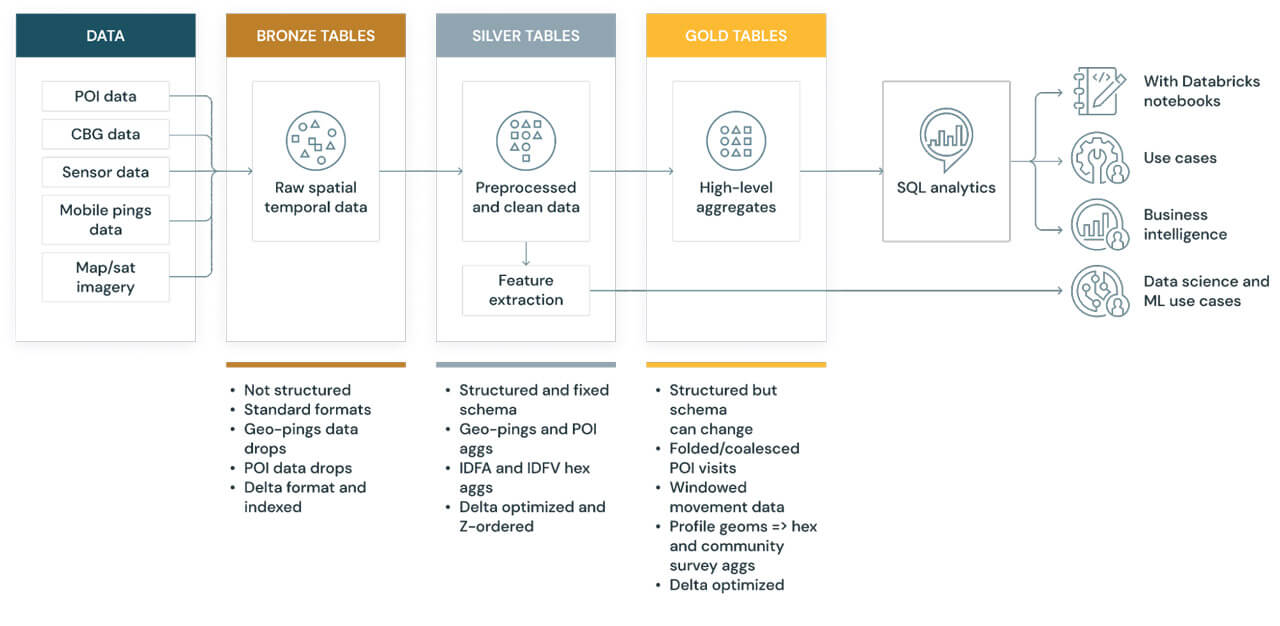
To your Geospatial Lakehouse, within the Bronze Layer, we suggest touchdown uncooked information of their “authentic constancy” format, then standardizing this information into essentially the most workable format, cleaning then adorning the information to greatest make the most of Delta Lake’s information skipping and compaction optimization capabilities. Within the Silver Layer, we then incrementally course of pipelines that load and be part of excessive cardinality information, multi-dimensional cluster and+ grid indexing, and adorning the information additional with related metadata to assist highly-performant queries and efficient information administration. These are the ready tables/views of successfully queryable geospatial information in a typical, agreed taxonomy. For Gold, we offer segmented, highly-refined information units from which information scientists develop and prepare their fashions and information analysts glean their insights, that are optimized particularly for his or her use instances. These tables carry LOB particular information for goal constructed options in information science and analytics.
Placing this collectively in your Databricks Geospatial Lakehouse: There’s a development from uncooked, simply transportable codecs to highly-optimized, manageable, multidimensionally clustered and listed, and most simply queryable and accessible codecs for finish customers.
Queries
Given the plurality of enterprise questions that geospatial information can reply, it’s essential that you simply select the applied sciences and instruments that greatest serve your necessities and use instances. To greatest inform these selections, you could consider the sorts of geospatial queries you intend to carry out.
Spatial k-nearest-neighbor be part of question (kNN-join question)
Spatio-textual operations
Libraries similar to GeoSpark/Sedona assist range-search, spatial-join and kNN queries (with the assistance of UDFs), whereas GeoMesa (with Spark) and LocationSpark assist range-search, spatial-join, kNN and kNN-join queries.
Partitioning
It’s a well-established sample that information is first queried coarsely to find out broader tendencies. That is adopted by querying in a finer-grained method in order to isolate all the pieces from information hotspots to machine studying mannequin options.
This sample utilized to spatio-temporal information, similar to that generated by geographic data techniques (GIS), presents a number of challenges. Firstly, the information volumes make it prohibitive to index broadly categorized information to a excessive decision (see the following part for extra particulars). Secondly, geospatial information defies uniform distribution no matter its nature — geographies are clustered across the options analyzed, whether or not these are associated to factors of curiosity (clustered in denser metropolitan areas), mobility (equally clustered for foot visitors, or clustered in transit channels per transportation mode), soil traits (clustered in particular ecological zones), and so forth. Thirdly, sure geographies are demarcated by a number of timezones (similar to Brazil, Canada, Russia and the US), and others (similar to China, Continental Europe, and India) aren’t.
It’s tough to keep away from information skew given the dearth of uniform distribution except leveraging particular strategies. Partitioning this information in a fashion that reduces the usual deviation of information volumes throughout partitions ensures that this information may be processed horizontally. We suggest to first grid index (in our use case, geohash) uncooked spatio-temporal information based mostly on latitude and longitude coordinates, which teams the indexes based mostly on information density reasonably than logical geographical definitions; then partition this information based mostly on the bottom grouping that displays essentially the most evenly distributed information form as an efficient data-defined area, whereas nonetheless adorning this information with logical geographical definitions. Such areas are outlined by the variety of information factors contained therein, and thus can symbolize all the pieces from giant, sparsely populated rural areas to smaller, densely populated districts inside a metropolis, thus serving as a partitioning scheme higher distributing information extra uniformly and avoiding information skew.
On the similar time, Databricks is growing a library, often called Mosaic, to standardize this method; see our weblog Environment friendly Level in Polygons through PySpark and BNG Geospatial Indexing, which covers the method we used. An extension to the Apache Spark framework, Mosaic permits simple and quick processing of huge geospatial datasets, which incorporates in-built indexing making use of the above patterns for efficiency and scalability.
Geolocation constancy:
Usually, the higher the geolocation constancy (resolutions) used for indexing geospatial datasets, the extra distinctive index values will probably be generated. Consequently, the information quantity itself post-indexing can dramatically improve by orders of magnitude. For instance, growing decision constancy from 24000ft2 to 3500ft2 will increase the variety of doable distinctive indices from 240 billion to 1.6 trillion; from 3500ft2 to 475ft2 will increase the variety of doable distinctive indices from 1.6 trillion to 11.6 trillion.
We should always all the time step again and query the need and worth of high-resolution, as their sensible functions are actually restricted to highly-specialized use instances. For instance, contemplate POIs; on common these vary from 1500-4000ft2 and may be sufficiently captured for evaluation properly under the best decision ranges; analyzing visitors at larger resolutions (masking 400ft2, 60ft2 or 10ft2) will solely require higher cleanup (e.g., coalescing, rollup) of that visitors and exponentiates the distinctive index values to seize. With mobility + POI information analytics, you’ll in all probability by no means want resolutions past 3500ft2
For one more instance, contemplate agricultural analytics, the place comparatively smaller land parcels are densely outfitted with sensors to find out and perceive effective grained soil and climatic options. Right here the logical zoom lends the use case to making use of larger decision indexing, given that every level’s significance will probably be uniform.
If a legitimate use case calls for top geolocation constancy, we suggest solely making use of larger resolutions to subsets of information filtered by particular, larger degree classifications, similar to these partitioned uniformly by data-defined area (as mentioned within the earlier part). For instance, when you discover a explicit POI to be a hotspot in your explicit options at a decision of 3500ft2, it could make sense to extend the decision for that POI information subset to 400ft2 and likewise for comparable hotspots in a manageable geolocation classification, whereas sustaining a relationship between the finer resolutions and the coarser ones on a case-by-case foundation, all whereas broadly partitioning information by the area idea we mentioned earlier.
Geospatial library structure & optimization:
Geospatial libraries differ of their designs and implementations to run on Spark. The bases of those elements drastically into efficiency, scalability and optimization in your geospatial options.
Given the commoditization of cloud infrastructure, similar to on Amazon Net Companies (AWS), Microsoft Azure Cloud (Azure), and Google Cloud Platform (GCP), geospatial frameworks could also be designed to reap the benefits of scaled cluster reminiscence, compute, and or IO. Libraries similar to GeoSpark/Apache Sedona are designed to favor cluster reminiscence; utilizing them naively, it’s possible you’ll expertise memory-bound conduct. These applied sciences might require information repartition, and trigger a big quantity of information being despatched to the motive force, resulting in efficiency and stability points. Operating queries utilizing most of these libraries are higher fitted to experimentation functions on smaller datasets (e.g., lower-fidelity information). Libraries similar to Geomesa are designed to favor cluster IO, which use multi-layered indices in persistence (e.g., Delta Lake) to effectively reply geospatial queries, and properly go well with the Spark structure at scale, permitting for large-scale processing of higher-fidelity information. Libraries similar to sf for R or GeoPandas for Python are optimized for a variety of queries working on a single machine, higher used for smaller-scale experimentation with even lower-fidelity information.
On the similar time, Databricks is actively growing a library, often called Mosaic, to standardize this method. An extension to the Spark framework, Mosaic gives native integration for straightforward and quick processing of very giant geospatial datasets. It contains built-in geo-indexing for top efficiency queries and scalability, and encapsulates a lot of the information engineering wanted to generate geometries from widespread information encodings, together with the well-known-text, well-known-binary, and JTS Topology Suite (JTS) codecs.
What information you intend to render and the way you goal to render them will drive selections of libraries/applied sciences. We should contemplate how properly rendering libraries go well with distributed processing, giant information units; and what enter codecs (GeoJSON, H3, Shapefiles, WKT), interactivity ranges (from none to excessive), and animation strategies (convert frames to mp4, native reside animations) they assist. Geovisualization libraries similar to kepler.gl, plotly and deck.gl are properly fitted to rendering giant datasets rapidly and effectively, whereas offering a excessive diploma of interplay, native animation capabilities, and ease of embedding. Libraries similar to folium can render giant datasets with extra restricted interactivity.
Language and platform flexibility:
Your information science and machine studying groups might write code principally in Python, R, Scala or SQL; or with one other language completely. In deciding on the libraries and applied sciences used with implementing a Geospatial Lakehouse, we want to consider the core language and platform competencies of our customers. Libraries similar to Geospark/Apache Sedona and Geomesa assist PySpark, Scala and SQL, whereas others similar to Geotrellis assist Scala solely; and there are a physique of R and Python packages constructed upon the C Geospatial Knowledge Abstraction Library (GDAL).
Instance implementation utilizing mobility and point-of-interest information
Structure
As offered in Half 1, the final structure for this Geospatial Lakehouse instance is as follows:
Diagram 1
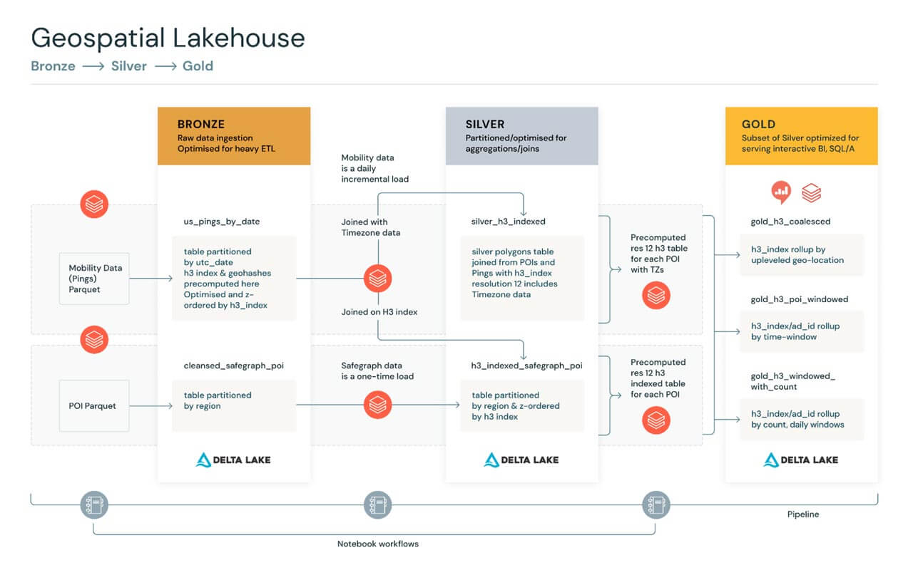
Making use of this architectural design sample to our earlier instance use case, we are going to implement a reference pipeline for ingesting two instance geospatial datasets, point-of-interest (Safegraph) and cell gadget pings (Veraset), into our Databricks Geospatial Lakehouse. We primarily deal with the three key levels – Bronze, Silver, and Gold.
Diagram 2
As per the aforementioned method, structure, and design rules, we used a mix of Python, Scala and SQL in our instance code.
We subsequent stroll via every stage of the structure.
Uncooked Knowledge Ingestion:
We begin by loading a pattern of uncooked Geospatial information point-of-interest (POI) information. This POI information may be in any variety of codecs. In our use case, it’s CSV.
Bronze Tables: Unstructured, proto-optimized ‘semi uncooked’ information
For the Bronze Tables, we rework uncooked information into geometries after which clear the geometry information. Our instance use case contains pings (GPS, mobile-tower triangulated gadget pings) with the uncooked information listed by geohash values. We then apply UDFs to remodel the WKTs into geometries, and index by geohash ‘areas’.
Silver Tables: Optimized, structured & fastened schema information
For the Silver Tables, we suggest incrementally processing pipelines that load and be part of high-cardinality information, indexing and adorning the information additional to assist highly-performant queries. In our instance, we used pings from the Bronze Tables above, then we aggregated and reworked these with point-of-interest (POI) information and hex-indexed these information units utilizing H3 queries to write down Silver Tables utilizing Delta Lake. These tables have been then partitioned by area, postal code and Z-ordered by the H3 indices.
We additionally processed US Census Block Group (CBG) information capturing US Census Bureau profiles, listed by GEOID codes to combination and rework these codes utilizing Geomesa to generate geometries, then hex-indexed these aggregates/transforms utilizing H3 queries to write down extra Silver Tables utilizing Delta Lake. These have been then partitioned and Z-ordered much like the above.
These Silver Tables have been optimized to assist quick queries similar to “discover all gadget pings for a given POI location inside a specific time window,” and “coalesce frequent pings from the identical gadget + POI right into a single file, inside a time window.”
# Silver-to-Gold H3 listed queries
%python
gold_h3_indexed_ad_ids_df = spark.sql("""
SELECT ad_id, geo_hash_region, geo_hash, h3_index, utc_date_time
FROM silver_tables.silver_h3_indexed
ORDER BY geo_hash_region
""")
gold_h3_indexed_ad_ids_df.createOrReplaceTempView("gold_h3_indexed_ad_ids")
gold_h3_lag_df = spark.sql("""
choose ad_id, geo_hash, h3_index, utc_date_time, row_number()
OVER(PARTITION BY ad_id
ORDER BY utc_date_time asc) as rn,
lag(geo_hash, 1) over(partition by ad_id
ORDER BY utc_date_time asc) as prev_geo_hash
FROM goldh3_indexed_ad_ids
""")
gold_h3_lag_df.createOrReplaceTempView("gold_h3_lag")
gold_h3_coalesced_df = spark.sql("""
choose ad_id, geo_hash, h3_index, utc_date_time as ts, rn, coalesce(prev_geo_hash, geo_hash) as prev_geo_hash from gold_h3_lag
""")
gold_h3_coalesced_df.createOrReplaceTempView("gold_h3_coalesced")
gold_h3_cleansed_poi_df = spark.sql("""
choose ad_id, geo_hash, h3_index, ts,
SUM(CASE WHEN geo_hash = prev_geo_hash THEN 0 ELSE 1 END) OVER (ORDER BY ad_id, rn) AS group_id from gold_h3_coalesced
""")
...
# write this out right into a gold desk
gold_h3_cleansed_poi_df.write.format("delta").partitionBy("group_id").save("/dbfs/ml/blogs/geospatial/delta/gold_tables/gold_h3_cleansed_poi")
Gold Tables: Extremely-optimized, structured information with evolving schema
For the Gold Tables, respective to our use case, we successfully a) sub-queried and additional coalesced frequent pings from the Silver Tables to supply a subsequent degree of optimization b) embellished coalesced pings from the Silver Tables and window these with well-defined time intervals c) aggregated with the CBG Silver Tables and rework for modelling/querying on CBG/ACS statistical profiles in the US. The ensuing Gold Tables have been thus refined for the road of enterprise queries to be carried out each day along with offering updated coaching information for machine studying.
# KeplerGL rendering of Silver/Gold H3 queries
...
lat = 40.7831
lng = -73.9712
decision = 6
parent_h3 = h3.geo_to_h3(lat, lng, decision)
res11 = [Row(x) for x in list(h3.h3_to_children(parent_h3, 11))]
schema = StructType([
StructField('hex_id', StringType(), True)
])
sdf = spark.createDataFrame(information=res11, schema=schema)
@udf
def getLat(h3_id):
return h3.h3_to_geo(h3_id)[0]
@udf
def getLong(h3_id):
return h3.h3_to_geo(h3_id)[1]
@udf
def getParent(h3_id, parent_res):
return h3.h3_to_parent(h3_id, parent_res)
# Observe that mum or dad and youngsters hexagonal indices might usually not
# completely align; as such this isn't meant to be exhaustive,
# reasonably simply reveal one kind of enterprise query that
# a Geospatial Lakehouse may also help to simply handle
pdf = (sdf.withColumn("h3_res10", getParent("hex_id", lit(10)))
.withColumn("h3_res9", getParent("hex_id", lit(9)))
.withColumn("h3_res8", getParent("hex_id", lit(8)))
.withColumn("h3_res7", getParent("hex_id", lit(7)))
.withColumnRenamed('hex_id', "h3_res11")
.toPandas()
)
example_1_html = create_kepler_html(information= {"hex_data": pdf }, config=map_config, peak=600)
displayHTML(example_1_html)
...
Outcomes
For a sensible instance, we utilized a use case ingesting, aggregating and remodeling mobility information within the type of geolocation pings (suppliers embrace Veraset, Tamoco, Irys, inmarket, Factual) with focal point (POI) information (suppliers embrace Safegraph, AirSage, Factual, Cuebiq, Predicio) and with US Census Bureau Group (CBG) and American Group Survey (ACS), to mannequin POI options vis-a-vis visitors, demographics and residence.
Bronze Tables: Unstructured, proto-optimized ‘semi uncooked’ information
We discovered that the candy spot for loading and processing of historic, uncooked mobility information (which usually is within the vary of 1-10TB) is greatest carried out on giant clusters (e.g., a devoted 192-core cluster or bigger) over a shorter elapsed time interval (e.g., 8 hours or much less). Cluster sharing different workloads is ill-advised as loading Bronze Tables is among the most useful resource intensive operations in any Geospatial Lakehouse. One can scale back DBU expenditure by an element of 6x by dedicating a big cluster to this stage. In fact, outcomes will differ relying upon the information being loaded and processed.
Silver Tables: Optimized, structured & fastened schema information
Whereas H3 indexing and querying performs and scales out much better than non-approximated level in polygon queries, it’s usually tempting to use hex indexing resolutions to the extent it’s going to overcome any acquire. With mobility information, as utilized in our instance use case, we discovered our “80/20” H3 resolutions to be 11 and 12 for successfully “zooming in” to the best grained exercise. H3 decision 11 captures a median hexagon space of 2150m2/3306ft2; 12 captures a median hexagon space of 307m2/3305ft2. For reference concerning POIs, a median Starbucks coffeehouse has an space of 186m2/2000m2; a median Dunkin’ Donuts has an space of 242m2/2600ft2; and a median Wawa location has an space of 372m2/4000ft2. H3 decision 11 captures as much as 237 billion distinctive indices; 12 captures as much as 1.6 trillion distinctive indices. Our findings indicated that the steadiness between H3 index information explosion and information constancy was greatest discovered at resolutions 11 and 12.
Growing the decision degree, say to 13 or 14 (with common hexagon areas of 44m2/472ft2 and 6.3m2/68ft2), one finds the exponentiation of H3 indices (to 11 trillion and 81 trillion, respectively) and the resultant storage burden plus efficiency degradation far outweigh the advantages of that degree of constancy.
Taking this method has, from expertise, led to whole Silver Tables capability to be within the 100 trillion information vary, with disk footprints from 2-3 TB.
Gold Tables: Extremely-optimized, structured information with evolving schema
In our instance use case, we discovered the pings information as sure (spatially joined) inside POI geometries to be considerably noisy, with what successfully have been redundant or extraneous pings in sure time intervals at sure POIs. To take away the information skew these launched, we aggregated pings inside slim time home windows in the identical POI and excessive decision geometries to cut back noise, adorning the datasets with extra partition schemes, thus offering additional processing of those datasets for frequent queries and EDA. This method reduces the capability wanted for Gold Tables by 10-100x, relying on the specifics. Whereas might have a plurality of Gold Tables to assist your Line of Enterprise queries, EDA or ML coaching, these will drastically scale back the processing instances of those downstream actions and outweigh the incremental storage prices.
For visualizations, we rendered particular analytics and modelling queries from chosen Gold Tables to greatest replicate particular insights and/or options, utilizing kepler.gl
With kepler.gl, we will rapidly render thousands and thousands to billions of factors and carry out spatial aggregations on the fly, visualizing these with completely different layers along with a excessive diploma of interactivity.
You’ll be able to render a number of resolutions of information in a reductive method — execute broader queries, similar to these throughout areas, at a decrease decision.
Under are some examples of the renderings throughout completely different layers with kepler.gl:
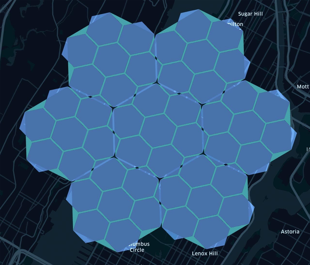
Right here we use a set of coordinates of NYC (The Alden by Central Park West) to supply a hex index at decision 6. We will then discover all the youngsters of this hexagon with a reasonably fine-grained decision, on this case, decision 11:
Diagram 3
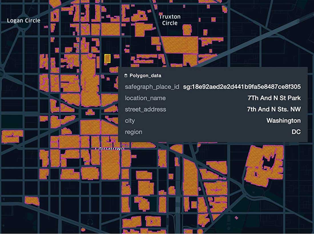
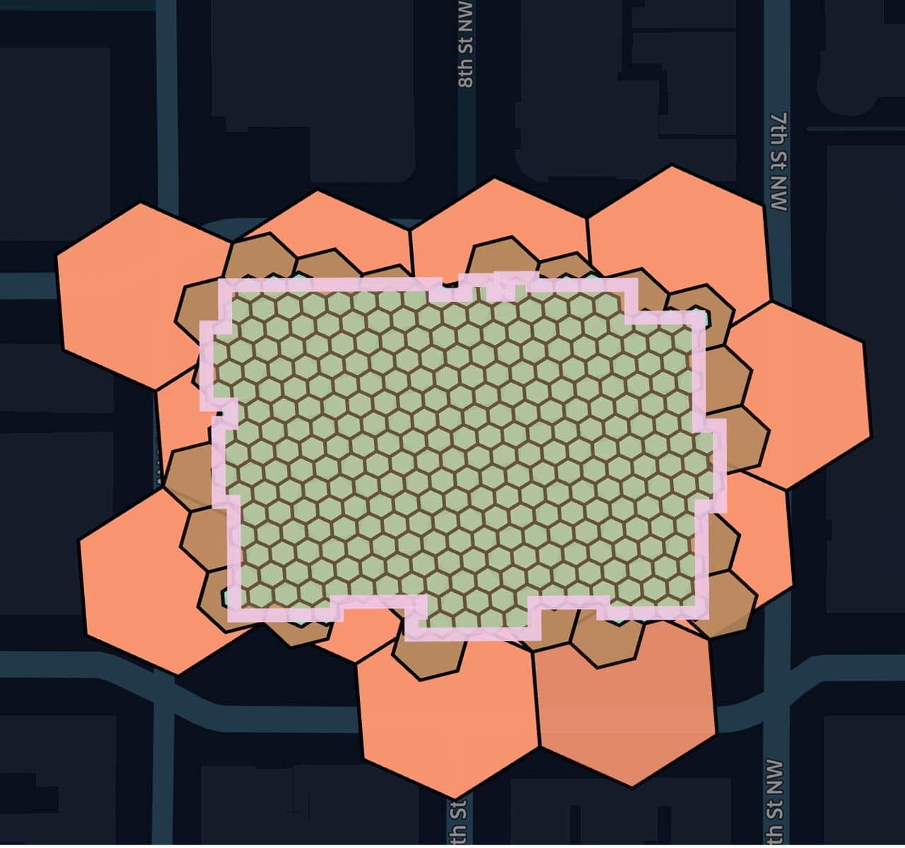
Next, we query POI data for Washington DC postal code 20005 to demonstrate the relationship between polygons and H3 indices; here we capture the polygons for various POIs as together with the corresponding hex indices computed at resolution 13. Supporting data points include attributes such as the location name and street address:
Diagram 4
Zoom in at the location of the National Portrait Gallery in Washington, DC, with our associated polygon, and overlapping hexagons at resolutions 11, 12 and 13 B, C; this illustrates how to break out polygons from individuals hex indexes to constrain the total volume of data used to render the map.
Diagram 5
You can explore and validate your points, polygons, and hexagon grids on the map in a Databricks notebook, and create similarly useful maps with these.
Technologies
For our example use cases, we used GeoPandas, Geomesa, H3 and KeplerGL to produce our results. In general, you will expect to use a combination of either GeoPandas, with Geospark/Apache Sedona or Geomesa, together with H3 + kepler.gl, plotly, folium; and for raster data, Geotrellis + Rasterframes.
Below we provide a list of geospatial technologies integrated with Spark for your reference:
GeoMesa ingestion is generalized for use cases beyond Spark, therefore it requires one to understand its architecture more comprehensively before applying to Spark. It is well documented and works as advertised.
Databricks Mosaic (to be released)
Spark 3
This project is currently under development. More details on its ingestion capabilities will be available upon release.
Scala/Java, Python APIs (along with bindings for JavaScript, R, Rust, Erlang and many other languages)
KNN queries, Radius queries
Databricks Mosaic (to be released)
Spark 3
This project is currently under development. More details on its indexing capabilities will be available upon release.
Visualization
We will continue to add to this list and technologies develop.
Downloadable notebooks
For your reference, you can download the following example notebook(s)
Raw to Bronze processing of Geometries: Notebook with example of simple ETL of Pings data incrementally from raw parquet to bronze table with new columns added including H3 indexes, as well as how to use Scala UDFs in Python, which then runs incremental load from Bronze to Silver Tables and indexes these using H3
Silver Processing of datasets with geohashing: Notebook that shows example queries that can be run off of the Silver Tables, and what kind of insights can be achieved at this layer
Silver to Gold processing: Notebook that shows example queries that can be run off of the Silver Tables to produce useful Gold Tables, from which line of business intelligence can be gleaned
KeplerGL rendering: Notebook that shows example queries that can be run off of the Gold Tables and demonstrates using the KeplerGL library to render over these queries. Please note that this is slightly different from using a Juypter notebook as in the Kepler documentation examples
Summary
The Databricks Geospatial Lakehouse can provide an optimal experience for geospatial data and workloads, affording you the following advantages: domain-driven design; the power of Delta Lake, Databricks SQL, and collaborative notebooks; data format standardization; distributed processing technologies integrated with Apache Spark for optimized, large-scale processing; powerful, high-performance geovisualization libraries — all to deliver a rich yet flexible platform experience for spatio-temporal analytics and machine learning. There is no one-size-fits-all solution, but rather an architecture and platform enabling your teams to customize and model according to your requirements and the demands of your problem set. The Databricks Geospatial Lakehouse supports static and dynamic datasets equally well, enabling seamless spatio-temporal unification and cross-querying with tabular and raster-based data, and targets very large datasets from the 100s of millions to trillions of rows. Together with the collateral we are sharing with this article, we provide a practical approach with real-world examples for the most challenging and varied spatio-temporal analyses and models. You can explore and visualize the full wealth of geospatial data easily and without struggle and gratuitous complexity within Databricks SQL and notebooks.
Next Steps
Start with the aforementioned notebooks to begin your journey to highly available, performant, scalable and meaningful geospatial analytics, data science and machine learning today, and contact us to learn more about how we assist customers with geospatial use cases.
The above notebooks are not intended to be run in your environment as is. You will need access to geospatial data such as POI and Mobility datasets as demonstrated with these notebooks. Access to live ready-to-query data subscriptions from Veraset and Safegraph are available seamlessly through Databricks Delta Sharing. Please reach out to datapartners@databricks.com if you would like to gain access to this data.